This guide was originally written as the introduction to my PhD thesis. I’ve gotten a lot of positive feedback from it and I think it deserves a wider readership, so I’ve reproduced it here. Errors, suggestions, questions, and comments can be submitted as GitHub issues, or you can find me on my socials.

Molecular Dynamics is a technique for computationally simulating a Newtonian approximation to complex chemical systems. It’s commonly used for studying protein folding and dynamics and modelling complex biochemical environments. In this guide, I’ll explain the basic statistical mechanics motivating MD, and also give some practical guidance on designing a computer experiment. I’ll shy away from giving explicit instructions on a particular software package.

Stat Mech and computers

Proteins as numbers

A computer requires a numerical representation of a protein to do any work on it. Most commonly, the protein’s state is recorded as a vector in so-called configuration space representing the positions of each atom, while the interactions between atoms are stored separately in a topology. The configuration space is an abstract vector space that spans all the possible combinations of positions of all the atoms in the system. Techniques that rely on velocities store them alongside the positions in a larger, but conceptually similar, ‘phase space’. Regions or points in these vector spaces correspond to states that the system could adopt.

It is also common to reduce the dimensionality of the system to make it easier to work with. This is called coarse-graining, in contrast to a detailed, fine-grained description. Common coarse-graining strategies include treating non-polar hydrogen atoms as part of their parent carbon atom (united-atom representation), treating water as a continuum rather than atoms (implicit solvent), or treating groups of atoms as single interaction sites. Indeed, treating the system as atoms can be considered a coarse-graining of a quantum chemical picture. The ultimate coarse-graining is to describe the entire system with a single variable, and this is commonly done; reaction coordinates, folding coordinates, concentration, temperature, pressure, and fluorescence intensity are all examples of this. In this way, coarse-graining can be thought of as the goal of all computational biophysics.

To give you a feel for what different representations of a protein might look like, here’s the mini-protein Chignolin at different levels of coarse graining. From left to right, quantum chemical representations model chemicals as nuclei and electrons; all-atom representations model them as bonds, bond angles, torsions, and atoms; united atom representations coarse grain hydrogen atoms into their associated heavy atom; and MARTINI (far right) combines four heavy atoms and their associated hydrogens into a single interaction site.

Statistical proteins

While we think of proteins as having a defined fold, they are far from static. The path they trace out in configuration space is extremely difficult to track, given the sheer number of configurations open to even a folded protein, and experiments do not give access to this path. Fortunately, chemical systems move so fast, and are so numerous in even a tiny amount of solution, that we can apply the law of large numbers and consider them statistically.

The statistical picture assigns every point in configuration space some probability density that represents how likely one is to find the system in that state. This forms a probability density surface over all of configuration space and gives any finite region of the space a finite probability. The system spends most of its time in regions of high probability, but occasionally traverses a barrier of low probability to move to a new region. These traversals constitute the dynamics of the system, with time-scales determined by the height of the barriers, and when different regions have different properties of interest we consider them different functional states. Many proteins have a small region of such high probability that it spends more time in this confined region than everywhere else put together, and we call that region the folded state. The size and structure of the region describes the dynamics of the folded protein.

Computational biophysics therefore estimates the shape of this probability surface for a particular system under some particular coarse graining and assumptions. The questions it is equipped to answer can always be posed in terms of a probability surface; for example:

• Structure prediction: Assuming there exists a unique high-probability structure, what is it?
• Rigid docking: Which ligand pose is most probable, assuming the protein doesn’t move?
• Mutation stability prediction: Which mutation will most improve the probability of this structure relative to some proxy of the unfolded state?
• Normal mode analysis: Assuming this structure is most probable, what other structures could this protein adopt?
• Reaction rate prediction: Assuming this path through phase space is important, how probable is it compared to doing nothing?

This statistical picture requires that the system be at equilibrium. Equilibrium can be broadly thought of as when the system has seen enough states that the law of large numbers applies and a statistical treatment is valid. At equilibrium, the probability density is well defined in terms of the energy via the Boltzmann distribution, as we will see shortly. There are several equivalent ways to define when a set of points in phase space, in the parlance an ‘ensemble of states’, is at equilibrium:

1. The probability density distribution does not depend on time;
2. the free energy is at a minimum;
3. the entropy is at a maximum;
4. net forward and reverse rates for all processes are equal;
5. there is no net work being done on or by the system.

While MD can in principle be applied out-of-equilibrium, other biophysical techniques generally cannot, and today’s computational models are generally parametrised at equilibrium. Fortunately, most properties of interest to structural biology are well defined at equilibrium, and many are simple averages over the equilibrium distribution. It’s worth noticing that this means that absolute rates (or kinetics) are generally not particularly accurate in MD; only the ratio of rates to their reverse rates are fitted with great care.

Probability from energy

We require some way to compute the probability distribution of a complex molecular system. Ideally, we would compute the distribution analytically, but analytical solutions generally do not exist except for very simple systems such as the ideal gas. Therefore, we must sample actual states from the distribution, generate an ensemble that represents a proportionate sample of states, and compute properties from that. In other words, the probability distribution must be computed numerically.

The equilibrium probability distribution of a molecular system at constant temperature is given by the Boltzmann distribution, which relates the probability of a state $P_i$ to the energy $\epsilon_i$: $$ P_i = \frac{\exp\left(\frac{-\epsilon_i}{K_BT}\right)}{Z} $$ Where $i$ indexes a state, some region (or point) in configuration space or phase space, coarse grained or otherwise; $\exp(x)$ is the exponential function $e^x$; $K_B$ is the Boltzmann constant; $T$ is the thermodynamic temperature; and $Z$ is the partition function, who we will meet shortly.

$\epsilon_i$ is an energy of state $i$, but its precise identity could be the potential energy, Gibbs free energy, or something else depending on both the thermodynamic ensemble and how the state is represented.

The partition function, $Z$, is simply the normalisation constant which ensures that the probabilities for all states sum to unity. It is a constant for a given chemical system under some specified conditions, or more technically one constrained to a particular region $S$ in phase or configuration space: $$ Z = \sum_{i \in S}\exp\left(\frac{-\epsilon_i}{K_BT}\right) $$

To see how the energy relates to the probability, we can take the natural logarithm and solve for the energy: $$ \epsilon_i = - K_BT \log(P_i) - K_BT \log(Z) $$ When $S$ represents all states available to a given system and temperature, we are at equilibrium, and $-K_BT \log(Z)$ is a constant called the free energy. We can also consider dividing, or partitioning, the phase space of a system into multiple regions or states ($S_0, S_1, …$). Each state is then distributed according to the Boltzmann distribution by considering the partition function of that state as though it were the whole system. Similarly, the free energy of the states can be computed from their respective partition functions. The whole system then obeys the Boltzmann equation, with $i$ indexing the sub-states and $\epsilon_i$ representing an energy of those states.

If we are content with relative energies between states of the same system, the zero of energy may be set to the partition function. Experiments generally only give relative energies so this is convenient, and it drastically simplifies computation: $$ \epsilon_{i\mathrm{rel}} = - K_B T \log(P_i) $$ In this view, energies are just a mathematically convenient representation of probabilities — the negative log likelihood. If several relative energies apply to a system, the total energy is simply the sum, consistent with multiplication for combining independent probabilities: $$ \epsilon_i + \epsilon_j = - K_B T \log(P_i P_j) $$ In addition, relative energies depend only on the interesting states — contributions of other states are thrown away with the partition function.

The probability and energy are therefore intimately linked. The energy of a state is proportional to the negative logarithm of the probability, and the constant of proportionality can be computed as the partition function of all the states accessible to the system. This proportionality constant cancels out when considering only relative states of the same system, which makes them a pragmatic abstraction in biophysics. Moving up a probability density surface is exactly equivalent to moving down the equivalent energy surface, albeit notably steeper thanks to the logarithm. If we can compute the appropriate energy of a state, we can thus easily draw conclusions about that state’s likelihood.

To illustrate the link between probability and energy, here are graphs of the probability and free energy surfaces of Chignolin along a simple one-dimensional folding coordinate. The other dimensions of configuration space are hidden in directions orthogonal to the page. The probability density (left) is a simple histogram of a converged REST2 simulation with the CHARMM22* force field; the free energy surface (right) is computed by taking the negative log likelihood, rescaling to units of kJ/mol, and subtracting a constant to set a convenient zero since I have not converged the partition function. You can see that relative to the probability density surface, the free energy surface is inverted and the local features are emphasised thanks to the negated logarithm function in the Boltzmann equation. The deep free energy minimum/probability density maximum at $x=0$ is the folded state!

When considering only configuration space properties under constant temperature, volume, and number of particles, the energy $\epsilon_i$ appearing in the Boltzmann distribution is simply the potential energy. In other conditions, the energy’s composition and identity differs. For phase space properties, the kinetic energy or temperature must be included in the energy. When the number of particles varies, the chemical potential must be included, and if the volume $V$ is allowed to vary in order to maintain a constant pressure $p$, the product $pv$ is included to account for work done by the system. Likewise, the energy depends on the representation of the state. Any region in a coarse-grained representation encapsulates some generally larger, higher dimensional region of the fine-grained configuration space, and the entropy available in interactions between such regions must be accounted for as potential energy in the coarse representation. Coarse-grained energy functions may be unable to faithfully reproduce these interactions if they rely on details that have been lost.

The energy surface

A 50 kDa protein with 500 residues, each of which can either be in an α-helix or β-sheet, has $2^{500}$, or about $10^{150}$, available states. At this coarse level of detail, only one state at most could be considered folded, and almost all states have steric clashes or otherwise high energies, and therefore low probabilities. If we were to search naïvely, the universe’s $10^{80}$ particles each computing a state every Planck time would take about $10^{19}$ years to find the folded state. This would be an inconvenient method for any biophysicist relying on sustainable power generation techniques, as all the stars in the universe will run out of fuel in only $10^{14}$ years.

This ludicrous two-state-per-residue representation is obviously insufficient. Real proteins even of much smaller size have many more possible states, firstly to model coil residues and non-ideal secondary structures, but also side-chains and solvents. How can we locate and score the reasonable structures without having to test every one of many possible states? Given this interpretation, nature’s ability to fold proteins in mere minutes or seconds is formidable. Computing the partition function might seem like a short cut, but in principle it requires converging a sum over all states and so takes just as long.

Nature solves this problem by letting the shape of the probability density guide its search. Most states have very high energies, and this leads to a near-zero probability after exponentiation, so only a tiny fragment of phase space is truly available to the system. As long as the potential energy surface is smooth enough, the system can flow down the surface to the regions of lowest free energy. In other words, a protein folds by following a funnel-shaped energy surface from any one of a huge number of unfolded states to a much lower number of folded states.

Here is a graphical representation of the funnel-shaped folding landscape of Chignolin; essentially the probability graph from the previous section expanded into a second dimension. Imagine the regions of high free energy (yellow) are level with the screen, and those of low free energy (blue) drop proportionally below it; the top of the funnel is sitting the plane of the screen, and it’s bottom is the blue area in the bottom left. The $x$-axis uses the same folding coordinate as previously (the distance between two atoms that form a hydrogen bond in the folded structure), while the $y$-axis uses the radius of gyration. Frames from the simulation are shown alongside their positions in the free energy surface.

We can see the two basic states of all proteins in this image; the folded state is the low energy, highly concentrated region in the bottom left ($x\approx0.0\ \mathrm{nm}, R_g\approx0.6\ \mathrm{nm}$), and the unfolded state is the rest of the surface, depicted in lighter colours, covering a wide variety of conformations including a prominent misfolded intermediate ($x\approx0.25\ \mathrm{nm}, R_g\approx0.6\ \mathrm{nm}$). The protein folds by falling into states of progressively lower free energy, which here most obviously form a shallow funnel from the broader unfolded state into the misfolded intermediate. From the misfolded state, the protein need only traverse a small energetic barrier to the folded state. The folded states’ high probability stabilises it even though there are many more states in the unfolded region, demonstrating the entropy-enthalpy trade-off. In addition, note the ruggedness of the surface; it is not a smooth funnel leading directly to the folded state, but meanders around and has many local minima.

Energy from state

Typical biophysical methods use some sort of function that goes from state to an energy-like quantity and is used to score the likelihood of structures. This is generally called a loss function or scoring function. The general procedure is then to search states until you find one that minimises the loss function. The loss function is the model of the interactions within the system, and the accuracy of the method is always limited to the true answer given the loss function, not that of reality.

Many physical laws are nothing more than functions that go from configuration to force. The force at a point $F(x)$ is simply the derivative of the potential energy:

$$ F(x) = \frac{∂}{∂x}U(x) $$

So it only takes a little integration to go from these physical laws to a potential energy! This can generally be done analytically. In the examples of Coulomb’s and Hooke’s laws:

$$ \begin{aligned} F(x) &= \frac{1}{4 \pi \epsilon_0} \frac{q_1 q_2}{x^2} \\ U(x) &= \frac{1}{4 \pi \epsilon_0} \frac{q_1 q_2}{x} \end{aligned} $$

$$ \begin{aligned} F(x) &= k x \\ U(x) &= \frac{1}{2} k x^2 \end{aligned} $$

The forces therefore give us a handle on the energies, and we can generally compute the energies as a function of the state.

Understanding energy as negative log likelihood can also be used in reverse to compute energy functions from known statistics, and energies are also often derived in a coarse-graining process from quantum chemistry. Machine learning has recently found enormous success in producing energy estimates when the system is represented in an appropriate basis.

However, a loss function alone can only give the relative likelihood of a state; to compute the absolute probability, we need some algorithm to provide context and find its place in the global probability distribution.

Choose your algorithm

If the energy surface, or model thereof, is simple enough, then well-known optimisation algorithms can very efficiently fold proteins. By combining a careful choice of representation with machine learning, AlphaFold won CASP13 with a learned probability density surface so smooth that it could be optimised just by starting at a point and iteratively moving in the direction with the steepest slope! This algorithm is called gradient descent. Hand optimised potentials like Rosetta commonly use variants of the Metropolis Monte Carlo sampling algorithm, which attempts to randomly change the system and then keep or retry the change depending on the change in the energy. A biophysical method therefore cannot be reduced to either its loss function or its algorithm.

Real proteins, and therefore highly accurate models of them, do not have potential energy surfaces smooth enough to optimise by gradient descent, which gets stuck in local minima before it can reach the folded state. Monte Carlo methods can, in principle, model the multi-state dynamics found in real proteins, but in practice simulating the dynamics of the system directly is more efficient because every change is guaranteed to be kept. This sampling procedure is known as molecular dynamics (MD). A machine learning approach that can sample directly from the Boltzmann distribution via a learned transformation from a Gaussian distribution has been developed; however even this method uses MD to generate training data.

Molecular Dynamics

The key insight behind molecular dynamics is that the same function can tell us about both the structure and dynamics of a physical system: the energy. In addition to being the negative log likelihood in configuration space, the potential energy’s derivative is the force, which models dynamics. This means that a function which simply computes the potential energy from the configuration can be differentiated in space to yield the forces on every part of the system. These forces can then be used to step the system through time, sampling the local energy surface. This function, called a force field, takes the place of a loss function in other techniques; it is where our knowledge about the world enters the simulation. Simulating the dynamics of a natural process is therefore a convenient way to sample phase space, not the goal of the technique.

There is a hidden assumption lying behind MD. For stepping through time to be equivalent to sampling, we must posit that averaging over time is equivalent to averaging over the equilibrium distribution. This is called the ergodic hypothesis, and a system where it is true is said to be ergodic. While ergodicity can be proved mathematically for simple systems, biomolecular systems are overwhelmingly too complex. Instead, ergodicity must be assumed from our intuition about the world and the fact that real proteins do, in fact, fold and equilibrate. If we take this step, and assume ergodicity, MD ceases to be mere simulation and instead becomes an efficient way to sample phase space.

MD is more efficient than other sampling methods for physical systems when there are many degrees of freedom. For example, Monte Carlo approaches to sampling a solvated protein in atomic detail must usually change only one atom per step and then compute the energy again, or else the step will most likely be rejected. MD allows every atom of a complex system to be moved in a way that guarantees acceptance. MD also is not limited by a library of possible moves; it enables arbitrary movement around phase space and guarantees that progress is made with every calculation. This is not to say that nature has stumbled upon the best algorithm for the problem; many so called enhanced sampling algorithms have been developed that use MD sampling at their core, but dramatically improve the efficiency by controlling where that sampling takes place.

While MD is routinely applied to small chemical systems using quantum mechanics to step through time, systems as large even as small peptides in explicit solvent must be approximated as Newtonian for efficiency. This treatment occurs at the level of atoms, usually as single interaction sites, because this is generally the smallest element of the system that it is reasonable to treat classically. While the corresponding gains in efficiency are enormous, Newtonian methods cannot describe processes that depend on quantum effects, such as the dynamics of individual electrons. As a result, chemical changes such as bond breaking or formation are generally inaccessible to classical MD.

The force field

A force field is a function $V(\bm{x})$ that yields the potential energy at coordinate vector $\bm{x}$ and is differentiable in $\bm{x}$. It encodes all the interactions and physical laws — except the laws of motion — of the system. Because it simply yields the potential energy, a force field is easier to parametrise than a scoring function; entropic free energy terms emerge spontaneously from the simulation, rather than being explicitly represented in the scoring function.

The negated derivative $\bm{F}(\bm{x})$ is a vector called the force: $$ \bm{F}(\bm{x}) = - \frac{∂}{∂x}V(\bm{x}) $$ The force field therefore not only encodes the potential energy, but also the forces. Force fields are usually constituted as the sum of individually differentiable terms, so the derivative can be computed analytically before a simulation. Force fields are extremely cheap to evaluate, both as energies and as forces, compared to both scoring functions and quantum chemical methods.

Today, force fields are simulated with periodic boundary conditions, which produce fewer modelling artefacts than walls or open boundaries. The system is constructed in a box, and atoms that leave one side of the box wrap around, re-entering the box from the other side. What is simulated is therefore a dilute liquid crystal of protein in water. Each pair of atoms is computed only once via the minimum image convention; only the interactions between an atom and its closest periodic image are calculated.

Modern force fields all use same basic mathematical functional form with different parameters, with some variance in how dihedral angles are treated. As an example, the CHARMM22* force field for a system of $n$ atoms is given as a potential energy function below: $$ V = \sum_{\mathrm{bonds}} k_b(b - b_0)^2 \; + \sum_{\mathrm{angles}} k_\theta(\theta - \theta_0)^2 \; + \sum_{\mathrm{cmaps}} \mathrm{cmap}(\phi, \ \psi) \\ + \sum_{\mathrm{dihedrals}} k_\phi(1 + \cos[\nu\phi - \delta]) \quad + \sum_{\mathrm{impropers}} k_\omega(\omega - \omega_0)^2 \\ + \sum_{i}^{n} \sum_{j}^{n} \left( \frac{1}{4\pi\epsilon_0}\frac{q_iq_j}{r_{ij}} \quad + \quad 4\epsilon_{ij} \left[ \left(\frac{\sigma_{ij}}{r_{ij}}\right)^{12} - \ \ \left(\frac{\sigma_{ij}}{r_{ij}}\right)^6 \right] \right) $$

The first two lines give the bonded potentials. $b$, $\theta$, $\phi$, and $\omega$ are respectively the values of a particular bond length, bond angle, dihedral angle or improper dihedral angle in the current state. $k_b$, $k_\theta$, $k_\phi$, and $k_\omega$ are their respective force constants, and $b_0$, $\theta_0$, $\phi_0$, and $\omega_0$ are their equilibrium values. $\nu$ and $\delta$ are respectively the dihedral angle’s multiplicity and phase, while $\mathrm{cmap}(\phi, \ \psi)$ is a function of the protein backbone dihedral angles $\phi$ and $\psi$ that maps a particular pair of values to an correction energy.

The last line represents the non-bonded potentials. $r_{ij}$ is the current distance between atoms $i$ and $j$, which is used in the pairwise Lennard-Jones and Coulomb potentials whose computation dominates the time spent calculating a force field on a state. $4\epsilon_{ij} \left[\left(\frac{\sigma_{ij}}{r_{ij}}\right)^{12}- \left(\frac{\sigma_{ij}}{r_{ij}}\right)^6\right]$ is the Lennard-Jones potential between atoms $i$ and $j$, parametrised by the energy well depth $\epsilon_{ij}$ and the distance $\sigma_{ij}$, which relates to the van der Waals radius $2^{\frac{1}{6}}\sigma_{ij}$. The Lennard-Jones potential models dispersion, van der Waals forces, and the Pauli exclusion principle. $\frac{1}{4\pi\epsilon_0}\frac{q_iq_j}{r_{ij}}$ is the Coulomb potential between atoms $i$ and $j$ with charges $q_i$ and $q_j$.

The CHARMM22* force field specifies not just this functional form, but also all of the parameters that go into it — that is, the symbols above that do not depend on the current state. The CHARMM27, CHARMM36 and CHARMM36m force fields share the same form with modified parameters, and other biomolecular force fields have only minor differences. Parametrising a force field requires the fitting of thousands of parameters to accurately reproduce many properties of interest, and requires substantial computational investment just in testing.

The non-bonded potentials account for the vast majority of computation during any MD step because they must be calculated for every pair of atoms in the system, which would lead the number of calculations to grow with the square of the number of atoms. This contributes to the substantial efficiency improvement achieved by coarse-grained force fields. These potentials are therefore truncated at 1.2 nm, and a shift is applied that smoothly reduces the forces and energies to zero at that cut-off, so that in practice the interactions can be computed in linear time.

Long-range Coulomb interactions can be important for biomolecular systems, so rather than using a cut-off, electrostatics can be computed efficiently for the entire periodic system in reciprocal space with methods such as particle mesh Ewald (PME). This allows long-range electrostatic interactions to act on proteins, and has been shown to be more realistic than other means of treating long-range electrostatics. Alternatives to PME include the similar Gaussian split Ewald method, used by the Desmond software; and the venerable reaction field, which replaces long-range electrostatics with a isotropic field of constant dielectric constant. Long-range interactions are usually not a problem for the Lennard-Jones potential as it decays much more quickly.

Sampling with dynamics

The unique formulation of a force field allows the system to be stepped through time. Given an initial state, forces and therefore accelerations are computed from the force field. Approximating the acceleration as varying linearly over a given time-step, the initial accelerations are the average acceleration over the time-step starting half a time-step before $t=0$ and ending half a time-step after. This is used to compute the velocity at half a time-step, and that velocity is similarly used to update positions at the full time step. This process is repeated, stepping the system through time. Symbolically for a single atom:

$$ \ddot{x}_t = \frac{F(x_t)}{m} $$ $$ \dot{x}_{t+\frac{1}{2}\Delta t} = \dot{x}_{t-\frac{1}{2}\Delta t} + \ddot{x}_t \Delta t $$ $$ x_{t+\Delta t} = x_{t} + \dot{x}_{t+\frac{1}{2}\Delta t} \Delta t $$

This algorithm is called the leapfrog integration algorithm and is a formulation of Newton’s equations of motion. It is called an integrator because as $\Delta t$ approaches 0, stepping through time like this becomes mathematically equivalent to integrating over time; it is therefore an example of a numerical integration algorithm. The leapfrog algorithm is an efficient, reversible, and symplectic algorithm that balances accurate integration with large time-steps.

With MD in hand as an efficient sampling method, rather than a simulation technique, there is room to improve its efficiency by making it less like a simulation. This is called enhanced sampling. Naïve MD is inefficient because most of its time is spent in regions of low energy and therefore high probability. Barriers between these regions are high in energy and transitions are rare, so the system can become trapped in local minima such as the initial state. By spending less computer time in areas that are frequently visited and somehow giving that time a greater statistical weight in the final ensemble, sampling can be dramatically accelerated.

Quantum MD also exists, but it is far too computationally expensive to be usable on proteins. Proteins are massive enough that they are well approximated by Newtonian mechanics, with a few exceptions. Critically, chemical reactions rely on the movement of electrons and cannot be treated classically, and will therefore not occur in classical MD. However, chemical reactions are easy to expect ahead of time and so their simulation can be avoided. Most other quantum effects are encoded in the force field as bond vibrations and the like. This treatment, essentially coarse-graining out electronic degrees of freedom, drastically simplifies the equations of motion and allows treatment of the system at an atomic level rather than having to consider electrons. This comes at the cost of a more difficult parametrisation when electron orbital shapes are important, for instance in metal binding proteins or when the effect of polarisation is significant.

Using Newton’s equations or the leapfrog algorithm alone would lead to the simulation sampling the micro-canonical ensemble, with a constant number of particles, volume and energy. The temperature and pressure is allowed to vary depending on equation of state $PV=nK_BT$. Real biochemical systems are coupled to heat baths that keep them at approximately constant temperature, for example the rest of the water in the beaker or solution in the pipette. The pressure is similarly stable. In order to sample from more realistic ensembles with a constant temperature or pressure, the integration algorithm can be modified with the addition of a thermostat or barostat, which might change the way velocities evolve to keep temperature constant, or make the box size dynamic to maintain steady pressure.

The trajectory

The output of a simple MD run is a series of points in phase space, each associated with a time, called a trajectory. These points, or frames, are highly correlated with the neighbours in time, so almost all of them are discarded for efficiency. It would usually be conservative to preserve one frame per picosecond with a time-step of two femtoseconds. This digital trajectory is a discrete approximation of the true trajectory, which is the unique continuous path through phase space that satisfies the equations of motion and starts at the simulation’s initial conditions.

Many-body systems like proteins are chaotic, so tiny changes in starting conditions lead to trajectories diverging exponentially with time. Identical starting conditions with theoretically deterministic algorithms can produce uncorrelated trajectories within nanoseconds of simulation time on different hardware due to differences in numerical rounding. With a finite time-step, the integrator also introduces integration error, further deviating it from the true trajectory. This error is ameliorated with a smaller time-step, and with a symplectic and reversible integrator the error approaches zero in the limit as the time-step goes to zero. So you should prefer a symplectic, reversible integrator.

While a short time-step may improve integration error, it also reduces sampling efficiency and therefore increases statistical error for a given amount of computational resources. Thus, it is not the case that the most rigorous simulations have the shortest time steps. It is generally clear when a simulation’s time step is too large, as the sudden, unrealistic changes in atom position from step to step violate assumptions made by the simulation software and lead to nearly immediate crashes. However, up to this point of instability, the sampling error almost always dominates and the largest possible stable time-step is therefore chosen. If extreme precision is required, a hybrid Monte Carlo scheme can eliminate integration error completely. There is also some hope that while the produced trajectory diverges from the true trajectory of the given starting conditions, it shadows, or approximates, some other starting conditions.

Ensembles from trajectories

The goal of MD is to generate an ensemble of states in proportion to their equilibrium probabilities. Such an ensemble differs in one significant way from a trajectory: structures in an ensemble are not associated with time. Properties that are independent of time and can be computed from the ensemble are called equilibrium, structural, or thermodynamic properties, whereas those that depend on time are called dynamical or kinetic. Modern force fields are optimised to reproduce good equilibrium properties, and minor improvements can dramatically improve kinetics for particular systems. MD algorithms such as thermostats, barostats and enhanced sampling methods are usually targeted at equilibrium properties and can disturb the kinetics of the system. Users should take extra care when investigating kinetic properties to ensure their method and force field are appropriate for the problem.

If our goal is to compute an ensemble, then it is important to remember that simulation is merely a means to that end. MD simulates the natural time-evolution of the system because it is an efficient means of sampling from the Boltzmann distribution, not because we want a video of a protein. While MD is reversible and deterministic in principle, in practice these are unimportant features of the method and most implementations discard them in favour of efficiency.

Simulations must be very long before they can produce more than a handful of statistically independent equilibrium samples. Microseconds of simulation of small soluble proteins is accessible on commodity hardware, and milliseconds on specifically designed hardware. Most proteins take milliseconds to minutes to fold, and important structures like amyloids take decades to mature. The statistical error associated with under-sampling the true equilibrium distribution at such disparate time-scales often silently dominates the results of a simulation and has probably contributed to MD’s reputation as being unreliable. In general, it is impossible to know in advance if something new would happen if we just simulated a little longer.

The statistical error can be improved by running many replicas of the simulation, each with different starting conditions. This is commonly done by starting many different simulations with the crystal structure, but different initial velocities. Their initial correlation will rapidly decay thanks to chaos, and after a short equilibration period one is left with an ensemble of independent trajectories. This ensemble weakens the reliance on the ergodic hypothesis and has been found to accelerate sampling for the same amount of simulation time. Plus, modern parallel computer hardware is often more efficiently exploited by numerous replicas that can be run independently than by a single simulation spanning across compute units.

Starting structures are usually not drawn from a force field’s equilibrium distribution. Modelling errors or artefacts from the starting structure, the differences between dilute solution and the environment of the crystal or the cell, errors in the force field or approximations made in preparing the system for simulation can all contribute to this. Because we wish to draw samples from the Boltzmann distribution, it is important to discard data collected before the system reaches equilibrium. Thermodynamic variables such as pressure, temperature, and energy usually stabilise faster than properties of interest, so it is important to test for equilibration for the property being measured. Automated methods are available.

With an ensemble of equilibrium trajectories in hand, properties can be computed from the trajectory as though it were an ensemble of states. When considering uncertainty, however, it is important to remember that frames in a trajectory are not statistically independent. Autocorrelation, convergence analysis, and bootstrapping can all provide estimates of the effective number of independent samples present in a trajectory for a given property. The Living Journal of Computational Molecular Science maintains a fantastic best practices guide for quantifying uncertainty and sampling quality.

An ensemble of states also gives direct access to entropic properties of the system. For a state with $\Omega$ equiprobable or degenerate microstates per unit volume in phase space, the entropy has a simple form: $$ S = K_B \log(\Omega) $$ That is, the entropy simply counts the number of specific atomic configurations that contribute to a state in some coarse-grained picture of the system. Loss function-based methods generally model proteins with single models, and so entropic effects must be directly modelled in the loss function as though they were a form of potential energy. Thus, effects like solvation and the hydrophobic effect, loop flexibility and entropic stabilisation of ligand binding must be parametrised directly. Molecular dynamics force fields produce ensembles rather than single models, and so these effects emerge from the dynamics of the potential energy surface.

Note that when microstates are not equiprobable, such as when the temperature is constant and energy is constantly exchanged with the environment, the entropy takes on a slightly more complex but conceptually similar form: $$ S = - K_B \sum_i{p_i \log(p_i)} $$ Where microstate $i$ has probability $p_i$. This so-called Gibbs entropy is equivalent to the Boltzmann entropy described above when all microstates have equal probabilities and unit volume in phase space.

The MD Cookbook

Force fields

Even with perfect sampling, MD only ever describes the world of the force field. If a problem is not within the force field’s narrow domain of applicability, the results may be irrelevant to the real world. Force field development has been going on for decades, but sufficient MD sampling to optimise them efficiently has only been available for less than a decade.

Proteins are the most important part of most biomolecular systems and are among the most difficult to parametrise. Thus, the choice of force field generally starts here. For another look at the state of the art, check out Thorben Fröhlking and colleagues’ preprint.

Openly accessible papers benchmarking the performance of protein force fields include:

• Lindorff-Larsen, K; Piana, S; Dror, R O Shaw, D E (2011) How fast-folding proteins fold, Science 334:6055 517–520
• Beauchamp, K A; Lin, Y-S; Das, R; Pande, V S (2012) Are protein force fields getting better? A systematic benchmark on 524 diverse NMR measurements JCTC 8:4 1409-1414
• Lindorff-Larsen, K; Maragakis, P; Piana, S; Eastwood, M P; Dror, R O; Shaw, D E (2012) Systematic validation of protein force fields against experimental data, PLoS ONE 7:2 e32131
• Fluitt, A M; de Pablo, J J (2015) An analysis of biomolecular force fields for simulations of polyglutamine in solution, Biophys J. 109:5 1009–1018
• Rauscher, S; Gapsys, V; Gajda, M J; Zweckstetter, M; de Groot, B L; Grubmüller, H (2015) Structural ensembles of intrinsically disordered proteins depend strongly on force field: A comparison to experiment, JCTC 11:11 5513–5524
• Petrović, D; Wang, X; Strodel, B (2018) How accurately do force fields represent protein side chain ensembles? Proteins 86:9 935–944
• Robustelli, P and Piana, S and Shaw, D E (2018) Developing a molecular dynamics force field for both folded and disordered protein states PNAS 115:21 E4758–E4766
• Sandoval-Perez, A; Pluhackova, K; Böckmann, RA (2017) Critical comparison of biomembrane force fields: Protein-lipid interactions at the membrane interface JCTC 13:5 2310–2321
• Cino, E A; Choy, W-Y; Karttunen, M (2012) Comparison of secondary structure formation using 10 different force fields in microsecond molecular dynamics simulations JCTC 8:8 2725–2740

CHARMM proteins

The CHARMM (CHemistry At Harvard Molecular Mechanics) force field family is distributed with the CHARMM MD software, and individual force fields are named for the version of the software they were first distributed with. They are parametrised with both structural information from quantum chemical calculations and experimental data. CHARMM22 was the first CHARMM all-atom force field for proteins. RNA parameters and dihedral correction maps were added in CHARMM27 (also called CHARMM22/CMAP), which improved backbone dihedral distributions. CHARMM27 has a notable bias for α-helix over β-sheet which was corrected in CHARMM36. CHARMM36m was then released to destabilise an unrealistic left-handed α-helix found in disordered proteins. CHARMM force fields are distributed by its authors in formats compatible with many different MD engines, making it a reliable parameter set that has steadily improved in quality and today approaches the state of the art.

There is one notable third-party optimisation of a CHARMM forcefield. CHARMM22* was produced after optimisation using orders of magnitude more sampling than previously available on the purpose-built Anton supercomputer. CHARMM22* abandons CHARMM27’s correction maps for backbone dihedral angles of residues other than glycine and proline with re-optimised dihedral parameters. It is a well-tested, accurate protein force field with excellent performance even on disordered proteins, despite being fitted exclusively to folded proteins.

Amber proteins

Amber force fields are distributed with the Amber software. Like CHARMM, they are parametrised with both QM and experimental data. New parameters are regularly released and rarely have time to be evaluated before they are updated. In addition, Amber force fields are a popular starting point for optimisations of force fields. ff99SB in particular has produced a popular and accurate family of force fields, beginning with an optimisation of the backbone parameters in ff99SB*. Later, several side chain dihedral potentials were improved and released as ff99SB-ILDN. These two improvements are commonly combined to form ff99SB*-ILDN, and an optimisation of atomic charges targeting per-residue helical propensities led to ff99SB*-ILDN-q. ff99SB*-ILDN-q was then optimised alongside the TIP4P-D water model aided by sampling from the Anton supercomputer to produce a99SB-disp, which includes both the protein and water parameters. Among other optimisations, a99SB-disp incorporates newly balanced water-protein dispersion forces to achieve a force field that accurately reproduces the properties of both folded and disordered proteins. a99SB-disp was also compared to several other modern force fields on benchmark systems that were not used in its parametrisation. Very recently, the protein–protein complex performance of a99SB-disp was further optimised with further Anton sampling to produce DES-Amber. This involved changes to the force field’s non-bonded parameters, and thus may be incompatible with other ff99SB-descended force fields.

Meanwhile, ff03 was developed on the basis of new quantum chemical calculations at a higher level of theory than the ff99SB family. Optimisations include ff03* and finally ff03ws. Inspired by ff99SB-ILDN, the Amber team derived ff14SB from ff99SB by re-parametrising backbone and side-chain dihedral parameters based on a large library of QM-optimised dipeptide conformations. ff14SB is the force field recommended by the Amber software team for all protein simulations. It was further optimised with a CHARMM-style dihedral correction map to improve performance with disordered peptides as ff14IDPs, and later ff14IDPSFF. The Amber team has also pursued a number of more systematic approaches to the production of force fields, resulting in ff14ipq, ff15ipq and FB15, though none of these have supplanted the traditional optimisation approach.

Many Amber-descended force fields have been found to be very accurate for folded proteins, especially those based on ff99SB-ILDN. Specific force fields have been optimised to reproduce methyl rotation barriers for NMR relaxation data, and NMR chemical shifts. Amber force fields also have access to a wide variety of parameters for non-canonical amino acids and post-translational modifications, and the free AmberTools software package provides extensive tooling for the parametrisation of new compounds.

GROMOS proteins

GROMOS force fields are parametrised to reproduce experimental thermodynamic energies and largely eschew structural properties from quantum chemical calculations. They use a united atom format, with non-polar hydrogen atoms coarse-grained with their parent carbon atom into a single interaction site. This reduces the number of atoms in the system but has been discarded as a strategy by other force fields because of its marginal effect in systems dominated by water and the increased flexibility provided by an all-atom model. The most recent GROMOS protein force field is GROMOS 54a7, and benchmarks have shown it to perform poorly on protein systems compared to recent CHARMM or Amber models. However, GROMOS does support a world-class automated topology builder for parametrisation of arbitrary molecules from automated QM calculations.

OPLS proteins

OPLS is an early force field with parameters for many classes of biomolecules. It was parametrised to reproduce experimental energies and QM structures. Protein parameters in the freely available version, OPLS-AA, has not been subject to the same level of optimisation as CHARMM and Amber. However, a commercially available release, OPLS3e combines OPLS’s broad molecule base with lessons learned from CHARMM and Amber regarding modelling proteins. It can produce results for protein-ligand binding energies with experimental accuracy for many drug-like molecules and is distributed with the commercial Schrödinger software. More recently, OPLS4 further improves performance.^ref

MARTINI

MARTINI is notable for being a coarse-grained force field. Instead of treating each atom explicitly, a single ‘bead’ represents approximately four heavy atoms along with their associated hydrogen atoms. This coarse-graining provides an approximately thousand-fold acceleration in sampling compared to atomic-resolution simulation. This enhanced performance derives not only from the reduced number of interactions, but also from an increased stable time-step $\Delta t$ and increased sampling owing to the smoother potential energy surface. While coarse-graining provides a substantial efficiency improvement, it comes at the cost of some loss in accuracy and precision.

MARTINI uses standard MD force field interactions and has a similar functional form to the above force fields, allowing it to run on existing MD software. Beads are organised according to their chemical properties, and multiple similar chemical groups can be represented by the same bead. Only integer charges are represented by electrostatics, and all other non-bonded interactions are realised with the Lennard-Jones potential. Rather than each bead being parametrised individually and pair potentials being derived from mixing rules as in other force fields, the matrix of Lennard-Jones interactions between all bead pairs is parametrised directly to reproduce experimental thermodynamic properties for simple molecules. Bonded parameters are then optimised against an atomic-resolution force field.

MARTINI was originally intended for simulations of lipids but has since been extended to other biomolecules including proteins, carbohydrates, and nucleic acids. The treatment of water has also been the subject of much optimisation, and tweaks have been made for GPUs, implicit solvent, or in combination with atomic-resolution models. The simplicity of the representation allows bead selection to be automated, making parametrisation of new molecules simple. MARTINI has been used to discover a new ligand binding pathway in the well-studied light harvesting complex II^ref and simulate entire viruses.^ref

Although MARTINI shines brightest when applied to massive systems on time-scales inaccessible to atomic-resolution MD, it can also be applied to smaller systems. The dynamics of individual proteins can be improved with an elastic network or by combining them with a structural Gō model. Protein parameters have been the subject of some optimisation already, and improved protein performance is a major goal of the recent MARTINI 3.0 update.^ref

MARTINI papers:

Unlike most other protein force fields, MARTINI is contributed to by groups around the world. This is probably because optimising a coarse grained force field is much more accessible than more detailed models, but is likely also due to the design of the force field itself. This has the upside of meaning that progress is made rapidly, but it also means that there’s a lot of literature to catch up on for the best models.

Fundamentals

• Marrink, Siewert J; Risselada, H Jelger; Yefimov, Serge; Tieleman, D Peter; de Vries, Alex H (2007-07-12) The MARTINI Force Field: Coarse Grained Model for Biomolecular Simulations., J. Phys. Chem. B 111:27 7812–24
• Marrink, Siewert J; Tieleman, D Peter (2013-08-21) Perspective on the Martini Model., Chem. Soc. Rev. 42:16 6801–22
• de Jong, Djurre H.; Baoukina, Svetlana; Ingólfsson, Helgi I.; Marrink, Siewert J. (2015) Martini Straight: Boosting Performance Using a Shorter Cutoff and GPUs, Comput. Phys. Commun.
• Alessandri, Riccardo; Souza, Paulo C. T.; Thallmair, Sebastian; Melo, Manuel N.; de Vries, Alex H.; Marrink, Siewert J. (2019) Pitfalls of the Martini Model, Journal of Chemical Theory and Computation 15:10 5448–5460

Lipid parameters

• López, César A.; Sovova, Zofie; van Eerden, Floris J.; de Vries, Alex H.; Marrink, Siewert J. (2013) Martini Force Field Parameters for Glycolipids, Journal of Chemical Theory and Computation 9:3 1694–1708
• Wassenaar, Tsjerk A.; Ingólfsson, Helgi I.; Böckmann, Rainer A.; Tieleman, D. Peter; Marrink, Siewert J. (2015-05-12) Computational Lipidomics with Insane : A Versatile Tool for Generating Custom Membranes for Molecular Simulations, J. Chem. Theory Comput. 11:5 2144–2155
• Marrink, Siewert J. (2018) Computational Modeling of Realistic Cell Membranes, Biophysical Journal 114:3 367a

Protein parameters

• Monticelli, Luca; Kandasamy, Senthil K.; Periole, Xavier; Larson, Ronald G.; Tieleman, D. Peter; Marrink, Siewert-Jan (2008-05) The MARTINI Coarse-Grained Force Field: Extension to Proteins, J. Chem. Theory Comput. 4:5 819–834
• Periole, Xavier; Cavalli, Marco; Marrink, Siewert-Jan; a. Ceruso, Marco (2009-09-08) Combining an Elastic Network with a Coarse-Grained Molecular Force Field: Structure, Dynamics, and Intermolecular Recognition, J. Chem. Theory Comput. 5:9 2531–2543
• Stark, Austin C.; Andrews, Casey T.; Elcock, Adrian H. (2013-09-10) Toward Optimized Potential Functions for Protein–Protein Interactions in Aqueous Solutions: Osmotic Second Virial Coefficient Calculations Using the MARTINI Coarse-Grained Force Field, J. Chem. Theory Comput. 9:9 4176–4185
• de Jong, Djurre H.; Singh, Gurpreet; Bennett, W. F. Drew; Arnarez, Clement; Wassenaar, Tsjerk A.; Schäfer, Lars V.; Periole, Xavier; Tieleman, D. Peter; Marrink, Siewert J. (2013-01-08) Improved Parameters for the Martini Coarse-Grained Protein Force Field, J. Chem. Theory Comput. 9:1 687–697
• Poma, Adolfo B.; Cieplak, Marek; Theodorakis, Panagiotis E. (2017-03-14) Combining the MARTINI and Structure-Based Coarse-Grained Approaches for the Molecular Dynamics Studies of Conformational Transitions in Proteins, J. Chem. Theory Comput. 13:3 1366–1374
• Javanainen, Matti; Martinez-Seara, Hector; Vattulainen, Ilpo (2017-11-13) Excessive Aggregation of Membrane Proteins in the Martini Model, PLOS ONE 12:11 e0187936
• Khan, Hanif Muhammad; Telles de Souza, Paulo Cesar; Thallmair, Sebastian; Barnoud, Jonathan; De Vries, Alex H.; Marrink, Siewert J.; Reuter, Nathalie (2020) Capturing choline-aromatics cation-π interactions in the MARTINI force field, Journal of Chemical Theory and Computation

Nucleic acid parameters

• Uusitalo, Jaakko J.; Ingólfsson, Helgi I.; Akhshi, Parisa; Tieleman, D. Peter; Marrink, Siewert J. (2015) Martini Coarse-Grained Force Field: Extension to DNA, Journal of Chemical Theory and Computation 11:8 3932–3945
• Uusitalo, Jaakko J.; Ingólfsson, Helgi I.; Marrink, Siewert J.; Faustino, Ignacio (2017) Martini Coarse-Grained Force Field: Extension to RNA, Biophysical Journal 113:2 246–256

Water models

• Arnarez, Clément; Uusitalo, Jaakko J.; Masman, Marcelo F.; Ingólfsson, Helgi I.; de Jong, Djurre H.; Melo, Manuel N.; Periole, Xavier; de Vries, Alex H.; Marrink, Siewert J. (2014) Dry Martini, a Coarse-Grained Force Field for Lipid Membrane Simulations with Implicit Solvent, Journal of Chemical Theory and Computation 11:1 260–275
• Michalowsky, Julian; Schäfer, Lars V.; Holm, Christian; Smiatek, Jens (2017) A refined polarizable water model for the coarse-grained MARTINI force field with long-range electrostatic interactions, The Journal of Chemical Physics 146:5 054501

Multiscale simulation

• Rzepiela, Andrzej J.; Louhivuori, Martti; Peter, Christine; Marrink, Siewert J. (2011) Hybrid simulations: Combining atomistic and coarse-grained force fields using virtual sites, Physical Chemistry Chemical Physics 13:22 10437
• Wassenaar, Tsjerk A.; Ingólfsson, Helgi I.; Prieß, Marten; Marrink, Siewert J.; Schäfer, Lars V. (2013-04-04) Mixing MARTINI: Electrostatic Coupling in Hybrid Atomistic–Coarse-Grained Biomolecular Simulations, J. Phys. Chem. B 117:13 3516–3530
• Zavadlav, Julija; Marrink, Siewert J.; Praprotnik, Matej (2019) SWINGER: A clustering algorithm for concurrent coupling of atomistic and supramolecular liquids, Interface Focus 9:3 20180075
• Liu, Yang; Pezeshkian, Weria; Barnoud, Jonathan; de Vries, Alex H.; Marrink, Siewert J. (2020) Coupling Coarse-Grained to Fine-Grained Models via Hamiltonian Replica Exchange, Journal of Chemical Theory and Computation 16:8 5313-5322

Automated parametrisation

• Bereau, Tristan; Kremer, Kurt (2015) Automated Parametrization of the Coarse-Grained Martini Force Field for Small Organic Molecules, Journal of Chemical Theory and Computation 11:6 2783-2791
• Graham, James A.; Essex, Jonathan W.; Khalid, Syma (2017) PyCGTOOL: Automated Generation of Coarse-Grained Molecular Dynamics Models from Atomistic Trajectories, Journal of Chemical Information and Modeling 57:4 650-656

Polarisable force fields

The force fields discussed above, with the exception of the polarisable MARTINI water model, are fixed-charge force fields. Fixed-charge force fields have a single, set charge value for each atom in the system that does not vary over the course of the simulation. Polarisation effects are parametrised implicitly in this charge, as well as in the bonded and Lennard-Jones parameters and in the dynamics of the water model. As most modern codes are tuned towards fixed-charge force fields, and since fixed charge force fields are much older and therefore more refined and better optimised, they generally yield better performance at present; for instance, polarisable force fields are not yet able to reliably produce folded protein structures from sequence alone. However, polarisable models are in development and may be necessary to obtain dramatic improvements over the state of the art in protein force field design.

Water models

The vast majority of any dilute biomolecular system is water, and solvent-protein interactions are very important to protein structure and dynamics. It is therefore essential that the water model used in protein simulations is both extremely fast and accurate in its interactions with the solute. Fortunately, the dynamics and structure of bulk water is less important and grants some flexibility for parametrisation. Ideally, a continuum model could be used in place of explicit water molecules, and work is being done in this direction especially by the Amber software. For the time being, an explicit solvent is much more accurate, and the best protein force fields are optimised around explicit solvent.

Solute force fields are optimised around particular water models, and care should be taken when using a different model. Therefore, it is safest to simply use the water model for which one’s protein force field is parametrised. Most protein force fields are parametrised for the 3-point water model TIP3P, although CHARMM uses a variant that includes Lennard-Jones interactions on all three atoms and GROMOS uses an alternative 3-point water model called SPC.

Several 4-point water models, with the oxygen’s charge moved to a fourth interaction site to simulate the lone pairs, have been parametrised for improved accuracy in different situations. These 4-point models are generally based on TIP4P. TIP4P-D^ref optimises the performance of disordered regions, which have been found to depend strongly on the precise strength of protein-water dispersion interactions. Unfortunately, it doesn’t reliably improve CHARMM22*, for which it was parametrised. TIP4P-Ew^ref was re-optimised for use with long-range electrostatics via PME rather than a Coulomb cut-off, similarly to the 3-point TIP3P-Ewald.^ref However, his appears to be an insignificant improvement, even where the effects of long-range electrostatics should be important.^ref TIP4P/2005^ref improves on the original TIP4P parameters with the benefit of twenty years of computer development, but requires re-parametrisation of the solute to improve protein performance.^refs a,b

Rather than optimising TIP4P, Izadi et al fitted the 4-point optimised point charge model (OPC)^ref by selecting charge locations that best reproduce the electrostatic field of water. This approach reproduces water’s bulk properties much better than models that locate charges on the hydrogen atoms,^ref and can also improve the performance of a TIP3P-optimised protein force field for intrinsically disordered proteins relative to other general purpose models.^ref 5-point water models, with interaction sites representing each of the oxygen atom’s lone pairs, improve the accuracy of the bulk water, but not the performance of solutes compared to 4-point models.^refs a,b

Metal cations

Organo-metallic binding is neither purely ionic nor spherically symmetric, and therefore the usual force field approximations of spherically symmetric potentials acting on atomic point charges without electronic structure or bond formation are naturally less appropriate. Nonetheless, fixed point charge models with optimised Lennard-Jones parameters are available with all force fields. These are generally appropriate for monovalent cations, but their performance degrades with divalent cations.^ref Multi-site models^refs a,b,c and modified potentials^refs a,b can improve the accuracy of divalent metal cations, but care should be taken when studying metal binding or when a metal is structurally important to a protein.

Drugs and small molecules

Proteins and nucleic acids have the advantage of being built up from relatively few building blocks. If the parameters of the building blocks are sufficiently accurate and transferable, then the whole macromolecule is accurate. Small, drug-like biomolecules exhibit a much wider variety of properties and structures, and therefore require enormously more parameters to describe accurately. Despite this, structural biology often relies on the interaction between small molecules and a protein. OPLS 3e claims similar accuracy to experiment with near-arbitrary drug molecules,^ref but is a proprietary, commercial force field with under-tested proteins. CHARMM has CgenFF^ref and Amber has GAFF,^ref both of which are general force fields designed to be transferable across different drug-like molecules. They do not require any QM calculation of the target in day-to-day use, making them convenient, but their accuracy leaves much to be desired.^refs a,b,c

In addition to the generalised parts of the GROMOS force field, the ATB^refs a,b is available to GROMOS users. Instead of being a generalised GROMOS-compatible force field, the ATB is an automated way to parametrise new molecules compatible with the existing GROMOS force field. It uses QM in parametrisation rather than relying on transferability and has shown greater accuracy and available chemical space compared to CgenFF or GAFF, but is much slower to parametrise taking hours rather than milliseconds per molecule. The ATB is available as a web server.

While still in its infancy, the Open Force Field Consortium^ref has developed a methodology of parametrising general force fields without atom types, dramatically simplifying the specification of the force field. SMIRNOFF99Frosst^ref is compatible with Amber force fields and has accuracy comparable to GAFF2 with only one tenth the number of parameters.^refs a,b It is hoped that this approach will lead to substantially more accurate general force fields in the near future.

Conclusion

The choice of force field is the most important step in an MD investigation, and the reliability of any results no matter how rigorously other steps are carried out are determined here. Fortunately, force field parameters for proteins have improved rapidly in recent years.

CHARMM22* is a reliable, well-tested force field for apo-proteins in salt water, or if accurate CHARMM parameters exist for any ligand. Amber ff99SB-disp or other descendants of Amber ff99SB*-ILDN also perform well, and are especially well suited to metallo-proteins and proteins with unusual amino acid residues when used with the appropriate additional parameters. OPLS 3e has excellent performance for drug-protein binding where it is affordable. Combining parameters between families of force fields should never be attempted, as different families have different strategies for computing non-bonded parameters and are not mutually compatible. Finally, the most reliable results are those that can be replicated or averaged across different high-quality force fields.

Sufficient sampling

Even if the force field perfectly models a phenomenon, one must have sufficient sampling to reach all the important states contributing to that phenomenon for the resulting ensemble to describe it. Furthermore, transitions between the important states must occur enough that the relative populations of the states has a reasonable uncertainty. There are many possible paths through configuration space, and an appealing narrative deduced from a single simulation may have very little to do with the real world or even the force field’s model.^ref It may be helpful to think of MD as a sampling technique, rather than a simulation technique.

Insufficient sampling can often, but not always, be revealed by assessing the uncertainty of quantities derived from simulation. This should be routine, as quantities should never be reported without uncertainty. However, computing the uncertainty from an MD simulation can be complicated by the fact that one cannot consider frames to be drawn independently from the underlying distribution. Grossfield et al ^ref have recently reviewed best practices in assessing uncertainty from trajectory data.

It is also important to consider expectations for a simulation; statistical approaches to uncertainty can only describe the uncertainty for regions of phase space that have already been reached. If a property’s true value is intermediate to contributions from two states, and a simulation is started in one of these states, the uncertainty will steadily improve with time as the state is fully explored. When the system makes a jump to the other state, the uncertainty will suddenly rise, despite the estimate of the property improving relative to the true value. The uncertainty may not fall to an acceptable level until many transitions between the two states have been observed. This is not an error, it merely reflects that there is no way to predict from a trajectory in one state alone that there exists a second important state. Thus, human intuition and insight is essential.

One potentially under-appreciated way to improve the robustness of sampling is to perform multiple replica simulations of the system.^refs a,b,c Not only does this improve utilisation of parallel hardware,^ref it also decreases the reliance on the ergodic hypothesis^ref and makes it easier to discard narratives that apply to only one simulation.^ref Empirically, 5-10 replicas is a good starting point, and one is generally better off splitting the same amount of computer time over many replicas rather than one long simulation.^ref

If one needs dramatically more sampling than is available with atomic-resolution simulation, a coarse-grained force field such as MARTINI^refs a,b should be considered. While the systemic errors introduced by this simplification may be substantial, they may be preferable to unknown statistical errors produced by under-sampling, especially for large systems.

Check your trajectory

Many errors resulting from unrealistic parameters and algorithms can be ignored by simulation software, but are quite apparent to a human observer. These can include (i) unphysical phase changes, such as frozen or evaporated water or gel-phase lipids; (ii) unexpected conformational changes, such as the rapid denaturation of proteins or loss of planarity in aromatic rings; (iii) vacuums spontaneously forming in condensed phase systems; (iv) violations of the second law of thermodynamics such as particle movement against concentration gradient. These errors can easily be carried forward throughout analysis and only noticed if they eventually cause an unbelievable result. It is therefore valuable to visually inspect simulations for such errors, at least until one has gained some level of confidence in their implementation of a method. One should also consider running automated validation tests on one’s system^ref that can detect non-Boltzmann sampling and other unphysical behaviour.

Choose software carefully

Much of the improvement in force fields of recent years may be attributed to a massive increase in the availability of compute hardware that is more appropriate to MD than the standard CPU. Three stand-out force fields (CHARMM22*, OPLS3e, and Amber ff99sb-disp) were all optimised with the Anton supercomputer, which was purpose-built to accelerate MD simulations by two orders of magnitude relative to the state of the art. At the same time, MD algorithms became available on GPUs, which had reached a price point at which a single GPU could perform an MD simulation faster than an entire cluster of CPUs. Purpose-built computer hardware is not within the reach of most researchers, but the great gains in efficiency accomplished by GPUs make their use nearly essential for MD today.

Statistical error usually dominates in MD simulations, so choosing an efficient platform is essential. Some codes have recently emphasised correctness, but most packages in use today are reasonably reliable, so it is generally best to use the fastest software and hardware that supports the desired method and force field. Changing software settings can make a substantial difference, so it is always useful to read the manual and understand how the simulation is executed by the software.

Popular codes today include:

1. GROMACS (GitHub), a free and open source package focusing on speed, flexibility, and recently safety;
2. Amber, a commercial package with great GPU and implicit solvent performance;
3. OpenMM (GitHub), a free and open source software library with extensive support for nearly arbitrary potentials at great speed;
4. NAMD, a fast and simple code that interoperates with popular visualisation software VMD; and
5. Desmond (free version), the free MD component of the proprietary Schrödinger software package whose commercial license includes the OPLS3e force field.

Boundaries and boxes

As it is impractical to perform a simulation of the entire universe, careful consideration must be applied to where in space a simulation ends and how these potentially discontinuous boundaries are treated. In biomolecular simulation with explicit solvent, periodic boundaries are used almost universally as they are simple to implement and produce minimal artefacts compared to alternatives like walls or open boundaries.

With periodic boundary conditions, the system is constructed in a triclinic box described by three box vectors. During simulation, the box is treated as though surrounded by copies of itself. Each atom has its copies separated from itself by integer multiples of the box vectors, and when one atom leaves the box in one direction it re-enters the box from the opposite side. Thus, the system is simulated in an infinite crystal lattice. This imposes some structure on the system as it is unable to move in ways that break this symmetry; however, this artefact is extremely mild for even moderately large boxes.

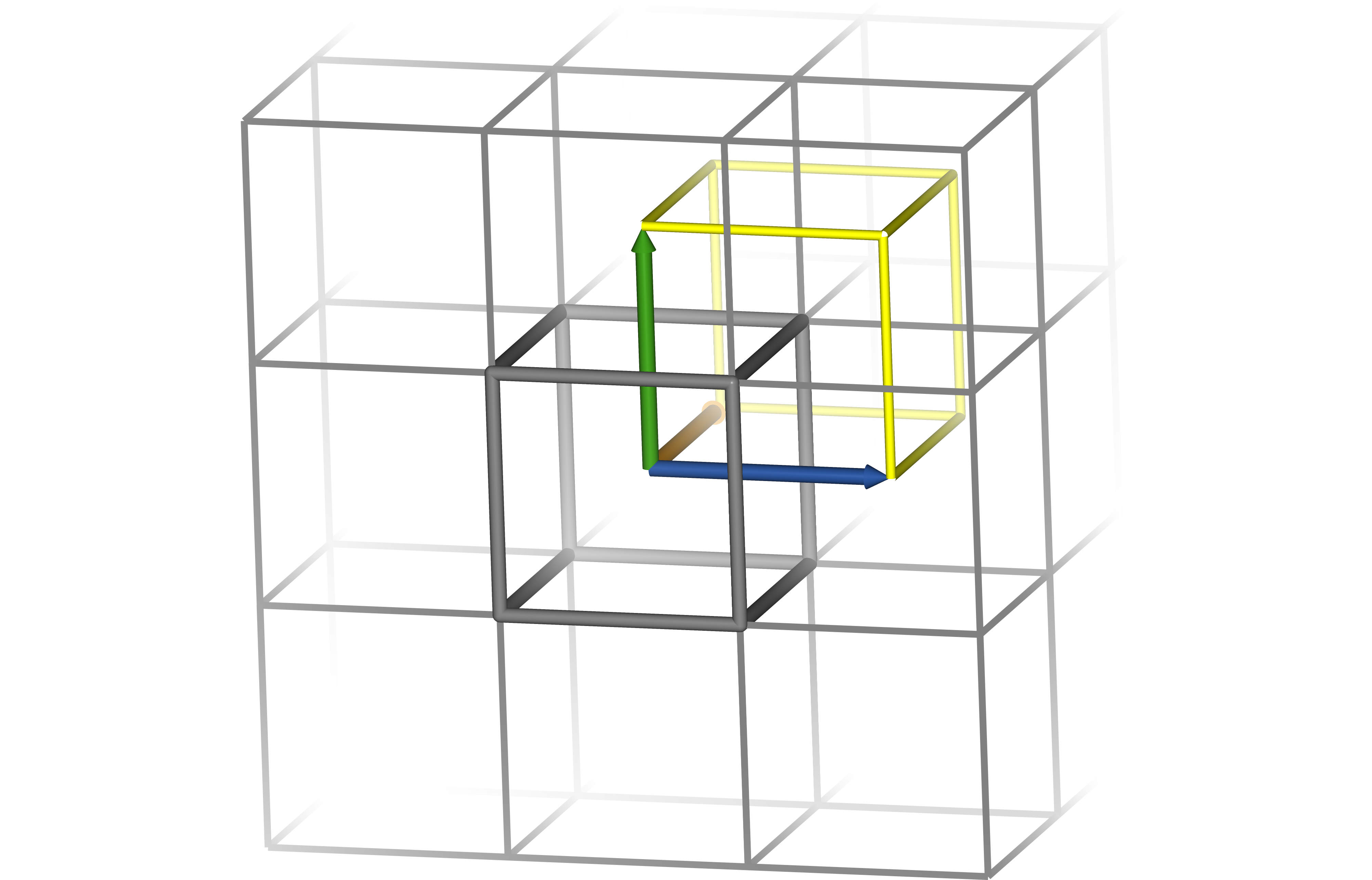
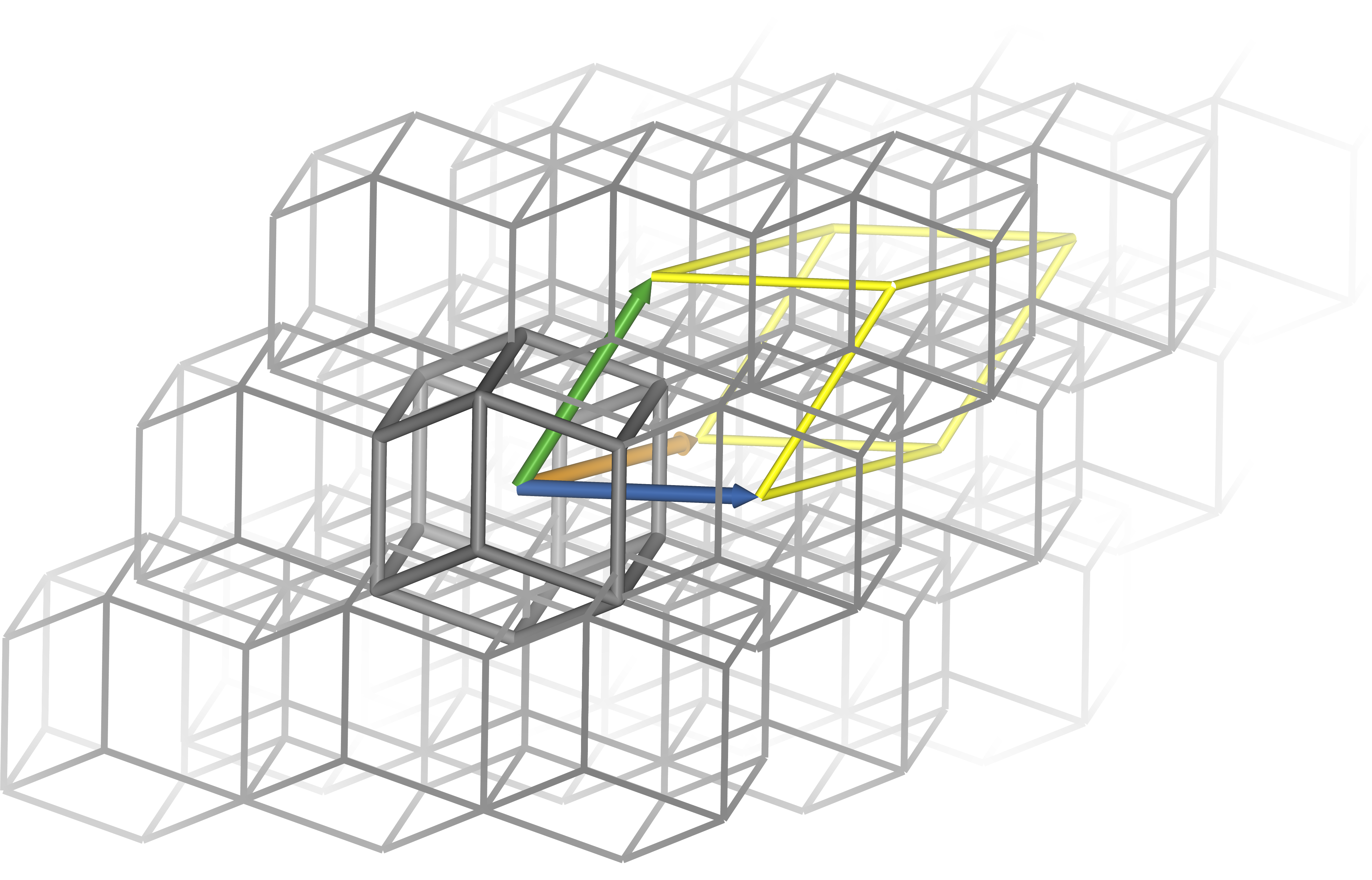
Below are diagrams of a cubic and rhombic dodecahedral boxes. Though the distance between a point and its image in the neighbouring cell is identical for both boxes, the rhombic dodecahedron has only about 71% of the cube’s volume. Blue, orange and green arrows indicate box vectors $\bm{a}$, $\bm{b}$ and $\bm{c}$. Grey lines indicate the edges of the box in its polyhedral representation. A single box is emphasised for clarity. Integer linear combinations of the box vectors translate coordinates from one box to another, and when centred on the origin the vectors outline one corner of the box’s triclinic representation (yellow lines) so that the centres of the polyhedra correspond to the vertices of the triclinic representation. Note that for the cube, the polyhedral and triclinic representations are identical, while for the rhombic dodecahedron they appear very different.

Periodic boundary conditions touch on almost every aspect of the simulation. The distance between two atoms is not uniquely defined, as both atoms exist in every box; by convention, the shortest such distance is used, which may not be the one in which both atoms share a box. Long-range electrostatic interactions are commonly calculated with Ewald methods such as PME that take advantage of periodic boundary conditions to efficiently compute every pairwise interaction in the box — and throughout the virtual crystal. If a constant pressure is required, the box size can even change over the course of the simulation, and this information must be propagated throughout the software.

There are also an infinite number of equivalent ways that the system of atoms can be represented. A common concern for new biophysicists is that bonds can appear to be broken across boundaries in the output trajectory, when in fact the output is simply an inconvenient representation of a physically correct system. Codes provide tools to change between these representations, but producing comprehensible representations of systems of multiple solutes can be difficult.

Because of this wide impact, the initial box size must be chosen carefully. Too small, and lattice artefacts become significant; too large, and simulation time is wasted on uninteresting solvent molecules. A common rule-of-thumb is that the solute should be separated from its periodic images by twice the non-bonded cut-off distance, or about 2 nm. It should be noted that this condition being satisfied at the start of the simulation does not guarantee that it will remain satisfied. Most importantly, proteins tumble on MD time-scales; this can be worked around by aligning the solute’s longest axis with the box’s shortest when computing the solvent buffer. Additionally, proteins can dramatically change shape through folding or conformational change, and constant-pressure simulations can experience changes in box size. As a result, Shabane et al recommend the box be at least four times the radius of gyration of a random coil model of the IDP.^ref

The shape of the box is also significant. While a cubic box is simple and traditional, a tumbling protein sweeps out a sphere, and so the corners of the cube are wasted. A rhombic dodecahedron is a triclinic box that can accommodate a spherical solute of the same size and with the same buffer as a cube with only 70.7% of the volume. This saves computer time by reducing the number of solvent molecules that must be simulated to fill the box. A rhombic dodecahedron with distance $d$ between an atom and its periodic image has box vectors: $$ \begin{aligned} \bm{a} &= \bigg\langle d, 0, 0 \bigg\rangle \\ \bm{b} &= \bigg\langle 0, d, 0 \bigg\rangle \\ \bm{c} &= \bigg\langle \frac{d}{2}, \frac{d}{2}, \frac{\sqrt{2} d}{2} \bigg\rangle \end{aligned} $$ If the greatest distance between two atoms in the solute is $l$, then $d$ can be estimated for a cut-off distance $r_c$: $$ d = l + 2r_c $$ Note that water models often have different densities, and a box containing poorly equilibrated solvent may contract or expand when pressure coupling is applied. In addition, this procedure will produce unnecessarily large boxes for systems that are expected to collapse over the course of the simulation, such as peptides in the extended conformation; for these, $d = l + r_c$ may be more appropriate.

Temperature and pressure coupling

Thermostats and barostats are the algorithm used to keep the temperature and pressure of a simulation constant. They modify the integrator to change the evolution of some other properties of the system, generally velocity or box size, in order to have deviations in the appropriate thermodynamic variables decay over time.

The choice of thermostat and barostat can have a substantial effect on the accuracy of a simulation. Because they modify the integrator, they will always have an effect on the dynamics of the system. Some thermostats and barostats do not produce the correct distribution of temperatures and pressures according to the appropriate ensemble, or have a larger impact on dynamics than an alternative.

Unexpected effects of coupling algorithms and some delightful horror stories can be found in these papers:

• Wong-ekkabut, J; Karttunen, M (2016) The Good, the Bad and the User in Soft Matter Simulations BBA Membranes 1858:10 2529–2538
• Basconi, J E; Shirts, M R (2013) Effects of temperature control algorithms on transport properties and kinetics in molecular dynamics simulations JCTC 9:7 2887–2899
• Braun, E; Moosavi, S M; Smit, B (2018) Anomalous effects of velocity rescaling algorithms: The flying ice cube effect revisited JCTC 14:10 5262–5272
• Rosta, E; Buchete, N-V; Hummer, G (2009) Thermostat artifacts in replica exchange molecular dynamics simulations JCTC 5:5 1393–1399
• Rizzi, A; Jensen, T; Slochower, D R; Aldeghi, M; Gapsys, V; Ntekoumes, D; Bosisio, S; Papadourakis, M; Henriksen, N M; de Groot, B L; Cournia, Z; Dickson, A; Michel, J; Gilson, M K; Shirts, M R; Mobley, D L; Chodera, J D (2020) The SAMPL6 SAMPLing challenge: Assessing the reliability and efficiency of binding free energy calculations J. Comput. Aided Mol. Des. 34 601-–633
• Rogge, S M J; Vanduyfhuys, L; Ghysels, A; Waroquier, M; Verstraelen, T; Maurin, G; Van Speybroeck, V (2015) A comparison of barostats for the mechanical characterization of metal–organic frameworks JCTC 11:12 5583–5597

Thermostats

Langevin dynamics

Langevin dynamics adds a randomly generated ‘friction’ term to the velocity of each atom during each integration step. This can be used to either model friction with the solvent in implicit solvent simulations, or heat exchange with the surroundings. In the latter case, the friction term becomes a thermostat. Langevin dynamics is well understood and easy to model, and molecular dynamics without a thermostat is often thought of as Langevin dynamics in the zero-friction limit.

CSVR thermostat (Author’s website)

The Canonical Sampling through Velocity Rescaling thermostat, also known as the Bussi or Bussi-Donadio-Parrinello thermostat, stochastically scales all the velocities of the simulation such that the total kinetic energy matches a value drawn from the appropriate ensemble. It can be thought of as Langevin dynamics, tuned to be minimally invasive, with a single random variable per step rather than one for each atom. It has been shown to be extremely efficient, reproducing canonical distribution temperatures with minimal disruption of dynamics and only one tunable parameter, and is a great choice for all simulations.

Nosé-Hoover chains

The Nosé-Hoover thermostat treats temperature as a virtual degree of freedom with its own equation of motion, and couples it to the velocities of the system. This was found to inhibit ergodicity for some systems and so was extended by Martyna and co-workers into a chained approach, which may still be problematic in replica exchange. It has the unique but dubious benefit of being deterministic, but is much more complex in its implementation than other temperature control algorithms.

Berendsen thermostat

This one’s historically important, but you shouldn’t use it. The Berendsen thermostat naïvely rescales velocities so that deviations in temperature decay at a user-configurable rate. It does not produce temperatures drawn from the canonical distribution, but is historically important as a predecessor to the CSVR thermostat that shares its strengths while being thermodynamically correct. Despite its violation of the equipartition principle, the many erroneous artefacts it has been found to introduce, and its inability to produce the correct ensemble, the Berendsen thermostat is still in wide use. The Berendsen thermostat has been superseded by CSVR and Nosé-Hoover chains and should not be used.

Andersen thermostat

The Andersen thermostat randomly reassigns the velocity of a single particle each integration step to a velocity drawn from the appropriate ensemble. In effect, this simulates collisions with the heat bath. While this is a simple method that produces the correct temperature distribution, it dramatically slows down kinetics — and therefore sampling — as particles all ‘forget’ their velocities over some short time period.

Alternate temperature control schemes

It has been proposed to use the solvent as a heat bath that doesn’t disturb dynamics at all, either by placing a thermostat only on the solvent or perhaps neglecting the thermostat altogether and using the solvent as a natural thermostat. These approaches have not proved popular and may be worth further exploration.

Barostats

Monte Carlo barostat

The Monte Carlo barostat is a family of barostats in which the box vectors are resized randomly, and then this change is either accepted or rejected according the Metropolis criterion. It is a simple barostat with rapid convergence properties that produces the correct ensemble. However, it abandons any notion of realistic pressure dynamics.

Berendsen barostat

The Berendsen barostat scales the box so that deviations from the target pressure vanish over some configurable time period. Like the Berendsen thermostat, this is simple and efficient but does not produce the correct ensemble. Its efficient convergence and stability makes it a popular choice in system equilibration, where rapid changes in box size are required, but it should not be used when collecting data.

Parrinello-Rahman and Martyna-Tuckerman-Tobias-Klein barostats

Similarly to the Nosé-Hoover thermostat, these barostats treat the pressure as an additional virtual degree of freedom coupled to box size and the positions of atoms. The MTTK barostat is an incremental improvement over PR; however, both are in wide use during data collection, especially when pressure dynamics are important. Both exhibit poor convergence properties, as large changes in box size can lead to oscillations and instability, and so should not be used when equilibrating the box size.

Stochastic Cell Rescaling barostat (Author’s website)

Similarly to the CSVR thermostat, stochastic cell rescaling incorporates random noise in rescaling the box to adopt the advantages and simplicity of the Berendsen barostat while being thermodynamically correct. While it has only recently been developed and is not yet widely available in efficient codes, it is likely to be a robust barostat for the same reasons that CSVR is. It is an anticipated feature of GROMACS version 2021.

Enhanced sampling

With the understanding that MD is first and foremost a convenient sampling technique for condensed-phase biomolecular systems, it becomes clear that simple integration algorithms may not be the most efficient. Enhanced sampling methods modify the basic dynamics of MD in various ways to accelerate sampling, either without altering the produced ensemble or by altering it in controlled ways that can be corrected in analysis. A wide variety of these methods were recently reviewed by Yang et al,^ref and LiveComSJ maintains a perpetual review of the field.

Simulated annealing^refs a,b

Simulated annealing is a widely applicable optimisation algorithm inspired by physics and later applied to molecular dynamics. At low temperatures such as the temperature of interest, sampling is in the correct ensemble but is very slow as high-energy transition barriers are only sampled rarely. At higher temperatures, sampling is faster but in the incorrect ensemble. Indeed, increasing the temperature is equivalent to decreasing the scale of every potential term in the force field, making it flatter and accelerating movement. Simulated annealing exploits this by performing sampling at the temperature of interest for some time, and then heating the system up to accelerate movement around the free energy surface. When the simulation is at a high temperature, data is not recorded, and sampling resumes when the system cools. This simple approach enhances sampling where it is slowed by having to negotiate energetic barriers in configuration space, as in biophysics.

Parallel tempering/temperature replica exchange^refs a,b

Parallel tempering, also known as temperature replica exchange (REMD), can be thought of as a parallel version of simulated annealing. Simulations of the same system are run in parallel at a range of temperatures like rungs on a ladder. With some frequency, adjacent replicas are allowed to swap coordinates according to the Metropolis criterion; that is, according to the Boltzmann probability that those coordinates would be found in each other’s ensemble. The replica at the temperature of interest is then used in analysis. It forms a discontinuous trajectory, with jumps around configuration space accelerated by trips to higher temperatures, but is entirely drawn from the appropriate ensemble and has dramatically less correlation between frames.

Efficiency of sampling can be assessed by the efficiency of movement around the temperature ladder,^ref so temperatures must be chosen that are close enough together that fluctuations in energy overlap. However, higher maximum temperatures also lead to greater efficiency, so many replicas may be needed.^ref Replica exchange is relatively simple to implement, and does not require specific knowledge about the system beyond the fact that sampling is slow because of enthalpic barriers.

When setting up a replica exchange simulation, a number of parameters must be chosen; the exchange frequency, the number of replicas, and the temperature ladder. There is some debate about how to choose the exchange frequency. In theory, exchange should be attempted very frequently for efficiency and is thermodynamically correct when done properly^refs a,b ; however, it has been suggested that in practice artifacts are introduced with exchange times below 1 ps,^refs a,b though this has not been shown with modern thermostats. The temperature ladder and number of replicas is simpler, however; the temperature ladder should be a geometric progression (though see also work by Gront and Kolinski^refs a,b ) starting at the temperature of interest and ending before the entropy dominates the free energy of interest, and the number of replicas should be chosen to maintain a respectable exchange acceptance ratio of about 20 – 30 %.^refs a,b,c

Hamiltonian replica exchange

Parallel tempering may be generalised by considering that temperature is not the only property that can affect sampling. Hamiltonian replica exchange uses a ladder with a modified energy function, or Hamiltonian, such that the bottom rung experiences normal sampling and the top rung’s sampling is substantially accelerated. The accelerated Hamiltonian is gradually turned on over the other rungs to permit exchange.

Since sampling only occurs on the unmodified bottom rung, any Hamiltonian that accelerates sampling and has an overlapping Boltzmann distribution can be used, even if it is physically nonsense. This allows the use of knowledge about the system to accelerate sampling while requiring many fewer replicas than parallel tempering. For example, heating up the water solvating a protein does not improve sampling, so parallel tempering can be improved by turning it into a H-REMD scheme that simply heats the protein.^refs a,b As many fewer atoms are heated in this scheme, the same sampling increase is achieved with many fewer replicas. Similarly, a model of the free energy surface along a slow coordinate can be used to sample other faster coordinates.^refs a,b

Bias methods

Bias methods are a large family of methods^{refs a,b,c,d,e,f,g,h} that vary greatly in detail but all work according to the same biophysical principles. Bias methods target a model of the free energy surface in terms of some coarse-grained low-dimensional coordinate system, or collective variable. Sampling along this variable is slow in simple MD because the trajectory dwells in regions of low free energy and cannot traverse large free energy barriers. A model of the probability distribution along the collective variable is built up on the fly from sampling done over the course of the simulation, and this is transformed into a energetic bias that is applied to the system. This boosts the system out of areas it has already explored and encourages it into new regions of phase space. Over time, as the model of the free energy surface becomes more accurate, sampling converges to uniformity across the collective variable.

Bias methods accelerate sampling along the collective variables they are applied to. If those collective variables describe the slowest degrees of freedom, then bias methods accelerate overall sampling. It should be noted that bias methods do not produce unbiased trajectories; instead, they produce a trajectory with a known time-dependent bias, as well as an unbiased model of the free energy surface in collective variable space. This model can be used to re-weight the trajectory, or as a bias for H-REMD.^ref Bias methods are also used alongside replica exchange methods to accelerate degrees of freedom for which collective variables are unavailable.^ref

These methods rely heavily on the choice of collective variable. If the wrong collective variable is chosen, stable convergence may be slow or the converged bias may not accelerate sampling overall. While this allows a researcher to leverage knowledge about the system to accelerate sampling, it is also prone to failure. Work has been done in the last several years to simplify and automate the selection of collective variables and even build them on the fly.^{refs a,b,c,d}

The most well known bias method is well-tempered metadynamics ,^ref in which Gaussians of slowly reduced size are added to the bias at the system’s current position with some frequency. Before it, umbrella sampling^ref involved placing harmonic biases along a collective variable and simulating the system independently in each in a sort of metadynamics-by-hand. Adaptive biasing force^ref is a bias method inspired by metadynamics and integrated into the Amber software package that uses a force-based spline as a bias. Supported similarly by GROMACS, the Accelerated Weight Histogram (AWH) method^ref uses a histogram to construct the bias. AWH differs notably by starting with a sweep across the entire collective variable space to rapidly converge a rough estimate of the bias that is then further optimised in additional sweeps. Both methods have a reduced overhead compared to metadynamics in their respective packages. Variationally Enhanced Sampling^ref formulates the construction of the bias as a minimisation problem, allowing great flexibility in the choice of biasing function. AWH and VES both support arbitrary target distributions defined in terms of their collective variables, allowing them to provide fine-grained corrections to an existing model.

Weighted Ensemble method

The Weighted Ensemble method is an extremely flexible, unbiased method that can be applied either to explore an unknown energy landscape^ref or to sample along a collective variable. The method exploits the fact that a rigorous re-sampling with re-weighting of a statistical ensemble preserves the distribution of the ensemble.^ref An ensemble of $n$ trajectories of the same system, each with an initial weight of $\frac{1}{n}$, are begun.^ref The simulations are run for a short time, then stopped. Trajectories that have reached interesting regions of configuration space are cloned, and their weights are divided among the children, while trajectories sampling regions of low free energy are culled and their weights concentrated on the survivors. This procedure is repeated and produces a swarm of weighted trajectory segments, which leads to an ensemble that converges rapidly in the ways defined as interesting. There is enormous flexibility in how simulations are re-sampled and which features are considered interesting,^ref and the method is easily applied to non-equilibrium systems.^ref

The weighted ensemble method is very similar to the popular Markov state model adaptive sampling approaches,^ref but does not rely on the assumption of Markovian dynamics. This makes it simpler, more flexible, and less error prone, and allows information coming from within a state to be retained in the final model. The method has been applied to an 11 minute process in 6 µs of simulation^ref and was reviewed recently by Zuckerman et al.^ref

Conclusion

MD has rapidly developed in the last decade since the application of GPUs to the problem of molecular simulation. Force fields have reached the point of reliability for soluble folded proteins, and are rapidly improving. Enhanced sampling methods are easy to use and continue to be worked on. As such, MD is reaching a level of maturity that permits its wide use by non-experts. Given the computational expense of performing an MD simulation, the complexity of the technique, and the plethora of features available from today’s software, users should be familiar with the goals and procedures of MD simulation. MD is sampling, not simulation; it is helpful to think of MD as a stochastic sampling method that produces states from an equilibrium ensemble, not a precise simulation of everything a system does from a given start point. This mindset reduces expectations that MD cannot yet meet, assists in choosing optimal parameters and methods, and emphasises the importance of a statistically rigorous interpretation of results.

Further Reading

Some great, freely available material to supplement this guide include:

• Justin Lemkul’s great GROMACS tutorials, which explain the mechanics of setting up a simulation in GROMACS
• The Best Practices papers, Tutorials and Training Articles, and Perpetual Reviews from the Living Journal of Computational Molecular Science (LiveComSJ), especially Best Practices for Quantification of Uncertainty and Sampling Quality in Molecular Simulations which details important information that isn’t covered in this guide.
• Peter Eastman’s fantastic Introduction to Statistical Mechanics